A lossless Compression technique
based on Discrete Radon Transform(s).
1. General principle
2. The very first results
2.2. Haar Mojette transform
2.3. Finite Radon Transform
3. Source code
4. References
The purpose of this page is to present and share the results of a collaboration between the
Image and Video Communication team (IRCCyN lab., Univ. Nantes, FRANCE) and the
School of Physics and Materials Engineering, Faculty of Science (Monash University, AUSTRALIA).
The people concerned so far by these researchs are:
- Florent Autrusseau (IVC-IRCCyN).
- Myriam Servieres (IVC-IRCCyN).
- Benoit Parrein (IVC-IRCCyN).
- Andrew Kingston (Monash Univ.).
- Imants Svalbe (Monash Univ.).
This work have been accepted for publication in ICASSP 2006.
If you want to use this work for your researchs, please cite:
- Florent Autrusseau, Benoit Parrein, Myriam Servieres, "Lossless Compression Based on a Discrete and Exact Radon Transform: A Preliminary Study", accepted for publication in the IEEE International Conference on Acoustics, Speech and Signal Processing, ICASSP'06, Toulouse, France 2006.
1. General Principle
We are currently trying to implement a compression scheme based on a projection transform (either the Mojette transform [1] from the IRCCyN lab, in Nantes, France, or the Finite Radon Transform (FRT) [2] used in the Monash University, Melbourne, Australia).
A few works in the IRCCyN lab focused on finding correlations WITHIN A Mojette projection, what we are working on now, is finding correlations BETWEEN several Mojette or FRT projections [3].
Here is the global idea :
Suppose you compute several Discrete Radon projections having very similar direction angles, you should obtain several very close projections (what we call bins).
We should then be able to first compute one mean projection, and then, to compute the difference between each bin value (of all projections) and the mean projection.
These projections being highly correlated, ideally, we should get very small difference values.
We would then just have to transmit or store the mean projection and all the (hopefully very small) difference projections, the so-obtained small differences projections could be encoded with only a few bits.
The first idea was to apply a Huffman compression technique on the differences projections.
This does reduce a little bit the amount of data, as we will see in the following.
We've also been thinking in applying statistical methods on the obtained projections, such as Principal Component Analysis (PCA) (Nothing's done yet on this topic).
Of course, an important problem we have to keep in mind with Discrete Radon Transforms is that we have to get exactly the right projections to process the inverse transform, otherwise, we will have very important back-projections errors (leading to encryption techniques, as shown in [4]).
This will probably cause important problems while applying PCA techniques.
We then have to apply a lossless compression technique on the 1-D projections.
Contrary to the FRT projections, the Mojette projections don't have the same length, then, the first thing we did from these projections, was to interpolate, in order to get all projections having the same length.
Figure 1 to 5 shows the results for image "boats" (of size 512x512).
Figure 1 shows the 7 projections (p,q= 1,75; 1,76; 1,77; 1,78; 1,79; 1,80; 1,81) obtained from the Mojette transform on a standard 512x512 grey level image.
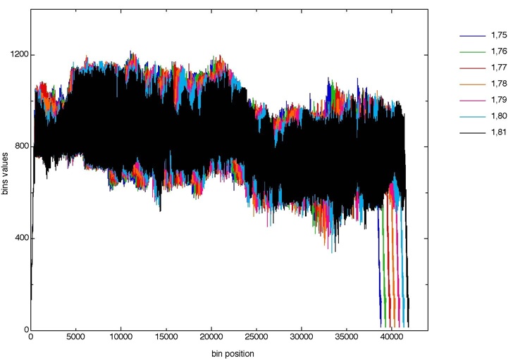
Figure 1. Mojette projections according to directions (1,75) (1,76) (1,77) (1,78) (1,79) (1,80) (1,81) before any interpolation.
Figure 2 shows the same projections after interpolation (to fit the highest number of bins - i.e. Nb of bins in the projection 1,81).
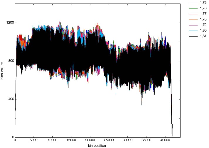
Figure 2. Mojette projections according to directions (1,75) (1,76) (1,77) (1,78) (1,79) (1,80) (1,81) after linear interpolati
And Figures 3 and 4 shows a detail of these curves (where the x-axis goes from 17400 to 17500).
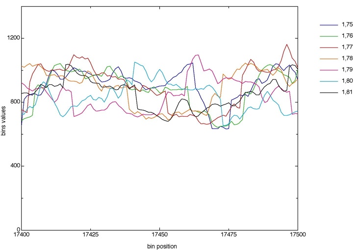
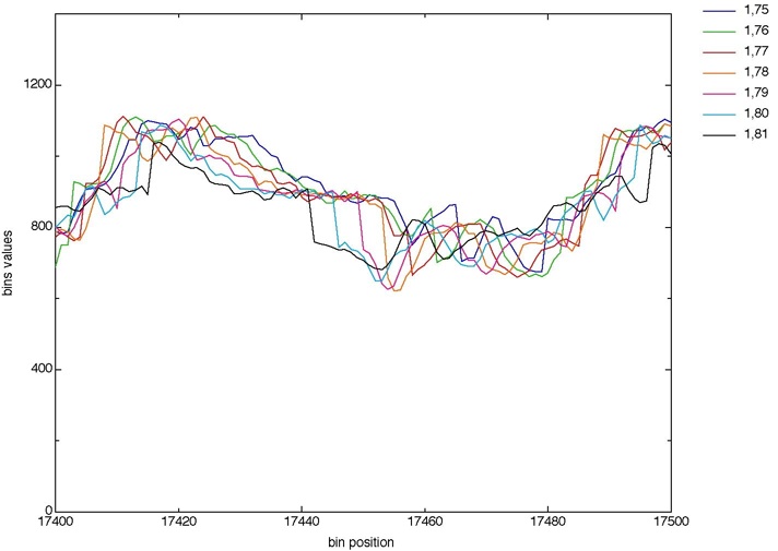
Figure 3. Zoom on the uninterpolated projections (from bin# 17400 to 17500).
Figure 4. Zoom on the interpolated projections (from bin# 17400 to 17500)
Figure 3 is a portion of the curves before interpolation (fig. 1), and figure 4 is part of the interpolated curves (fig. 2).
Note that the interpolation technique used here is the simplest one (linear interpolation).
Using more complex ones (bicubic, ...) might provide an even better correlation.
This clearly appears on Figure 4, where a little shift of the curves on the x-axis would induce a much better matching, and strongly reduce the difference projections.
Figure 5 also shows a part of the interpolated curves, but in a much larger range than fig 4.
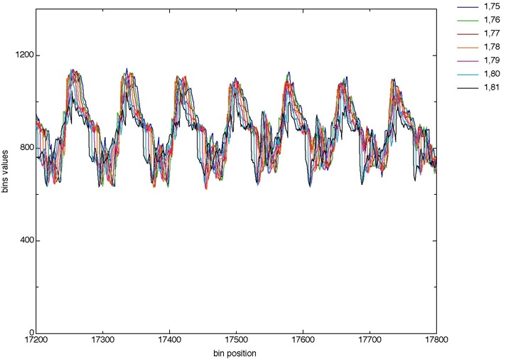
Figure 5. Another Zoom (different range: bins# 17200 to 17800).
Besides the compression aspect, this could be very useful in an encryption technique as well (as explained later).
This would allow to encrypt just a very small amount of information (the mean projection only, i.e. roughly 40000 bins in this case), instead of the whole image (262144 pixels), and transmit the encrypted mean projection along with the unchanged difference projections (which won't help without the original mean projection).
The program computing the entropy gives as an output file, the number of occurrences, i.e. for each, bin value, we know the overall number of bins equalling this value. See Figure 6. for an example.
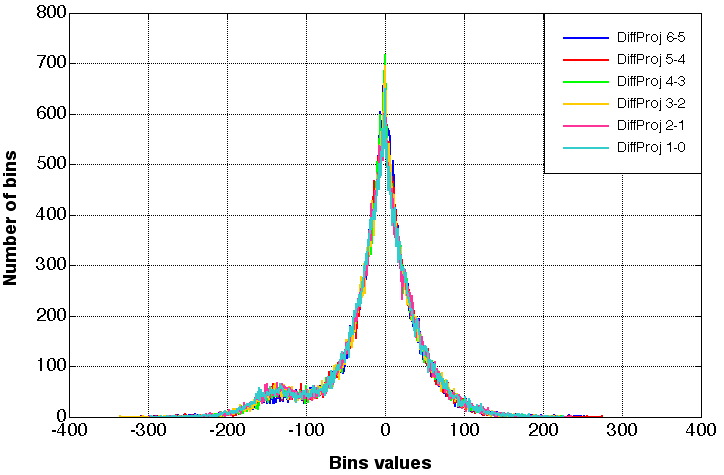
Figure 6a. Number of bins occurrences for the 6 difference projections
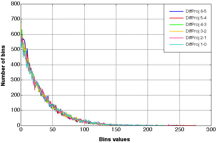
Figure 6b. (Zoom on) Number of bins occurrences for the 6 difference projections
2. The very first results
2.1. Dirac Mojette transform
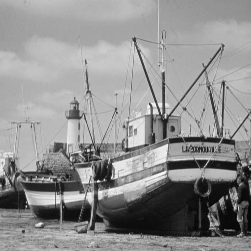
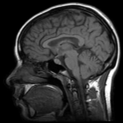
First of all, here are the four test images used in the following.
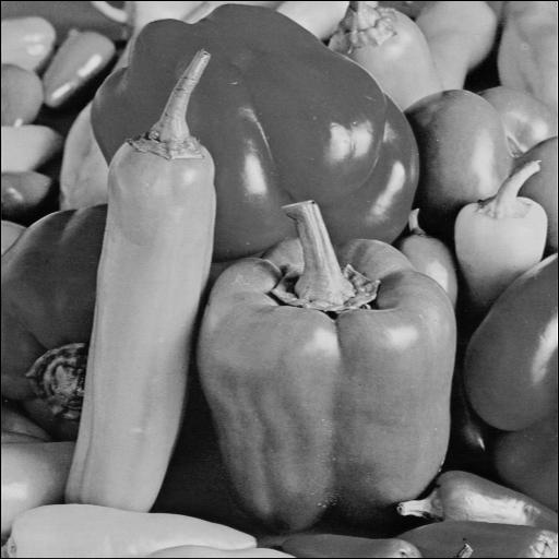
For the "peppers" test image, (of size 256x256 pixels, 8 bits per pixel).
and for the (1,128) and (1,129) projection angles.
We first computed these projections on the original image, we then computed the difference between these projections for each single bin, and finally, we computed the entropy for one original projection (1,129), as well as the entropy of the difference projection.
For one projection, the entropy gives the minimum amount of information we can use to encode this given projection.
So far, the idea to compress, is to process a Huffman encoding onto the projections, but maybe some other compression techniques could be better...
(We have to keep in mind though that the compression must be reversible.)
We also envisioned to combine Run Length Encoding (RLE) with Huffman coding for different projection angles, such as (127,128) and (128,129), where the Mojette transform provides a huge amount of bins equalling zero.
For the difference projection, we obtained an entropy of 5,22 bits per bin (bpb), while the entropy of the (1,129) projection was 8,15 bpb.
The projection length was 33151 bins, which means that if we want to transmit one original projection (the 1,129) along with the difference allowing to compute the other one (1,128), this gives a (minimum) total amount of :
(33151 bins x 8,15 bpb) + (33151 bins x 5,22 bpb) = 443 228 bits
instead of
256 x 256 x 8 bpp = 524288 bits
for a 8 bits per pixel image.
This means that we could remove approximately 15,46 % of the image information in a lossless compression technique.
(except that here, the Huffman dictionary size isn't included, this latter shouldn't be very important).
We also ran all this experiment on medical images and obtained very promising results, as there's a lot of zero value pixels.
The "mri" image provided 4,78 bpb for the difference projection, and 7,46 bpb for the original projection, which makes a total of :
(33151 bins x 7,46 bpb) + (33151 bins x 4,78 bpb) = 405 768 bits,
which means a suppression of 22,60 % of the data.
NOTE that this does NOT take into account the intr-projection coding (as explained later).
This coding reduces a little bit more the compression rate.
For real images, this might not be as good as for other well known lossless compression techniques (such as JPEG2000), but we can propose a few other services.
We could for instance compute 4 projections (with similar angles), encrypt only the mean projection, and send this encrypted projection along with the 4 unchanged difference projections. This would allow a very fast encryption algorithm, because we only encrypt a small projection instead of the whole image.
Furthermore, if we can increase the compression rate, we could have a joint source channel encoding technique : a compression technique ensuring data redundancy.
However, we believe that we could get better compression results, by simply applying a more adapted interpolation technique.
As seen in the first section, the Mojette transform gives projections of different length depending on the chosen angle, we then have to stretch the smallest projection, in order to compute the difference between the projections.
See for example on Figure 7, how the difference projection could be sensibly smaller by simply slightly shifting on the left the (1,129) projection (the difference is depicted in Figure 8).
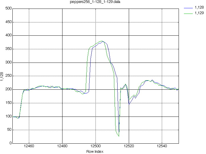
Figure 7. projections (1,128) and (1,129) for the image peppers (of size 256x256) (Zoom from bin# 12450 to 12550).
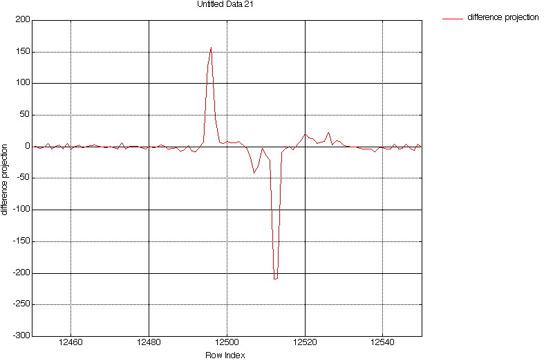
Figure 8. Difference between projections (1,128) and (1,129) for image "peppers" (Zoom from bin# 12450 to 12550).
As the FRT projections wouldn't require this interpolation (all these projections will have the same size), we expect very interesting results by using the FRT.
So far, we only ran the tests on grayscale images, but we could also use color images, the same algorithm would be applied on the Red, Green and Blue components.
Maybe in the future, we'll try to correlate the projections of different chromaticity components.
Finally, by having a look to the projections, we also figured out that they often represent similar sequences (see Figure 9).
Maybe a wavelet decomposition of the projections could be helpful ?!...
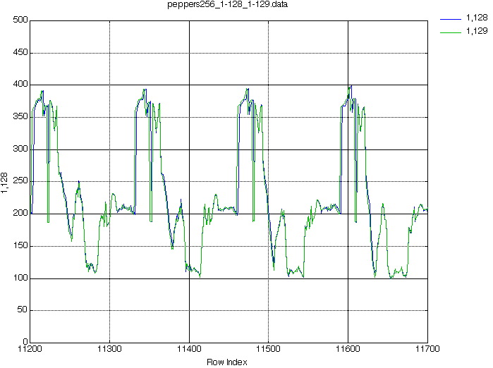
Figure 9. Larger Zoom on the two previous projections (from 11200 to 11700).
We can take advantage of such periodicity by simply encode the difference between each period.
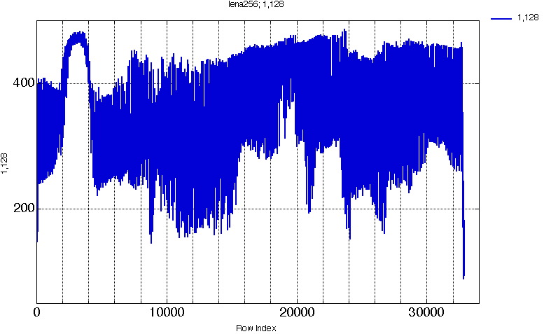
Figure 10. Projection (1,128) for image "lena" 256x256.
Fig. 10 shows the full projection for image lena, (p=1, q=128), this gives 32896 bins.
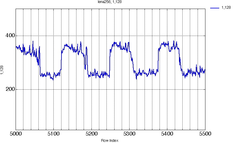 Figure 11a. 5000 -> 5500 |
|||
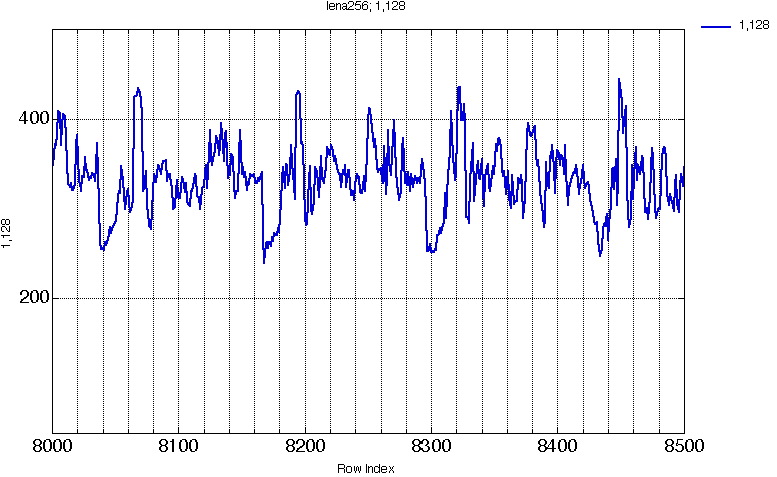 Figure
11b. 8000 -> 8500
|
|||
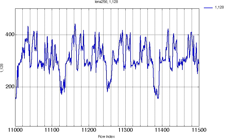 Figure 11c. 11000 -> 11500 |
|||
 Figure
11d. 15000 -> 15500
|
|||
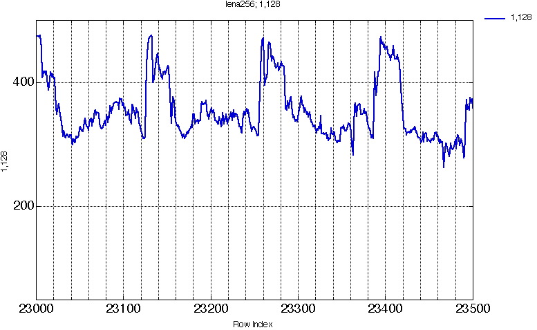 Figure 11e. 23000 -> 23500 |
|||
|
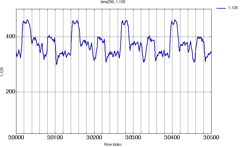
This was not obvious on the whole projection representation (Fig10.).
The period here equals q (=128), because the projection of two (horizontally) neighbor pixels are separated by q bins on the projection.
(Two vertically neighbor pixel, would be separated by p bins on the projection).
Hence, an efficient encoding algorithm can be implemented here.
We can compute a difference projection, by simply shifting a 128 bins large window over the whole projection, and get the difference of each couple of bins separated by q.
The Intra-projection difference corresponding to Fig 11a (from bin # 5000 to bin # 5500) is given below
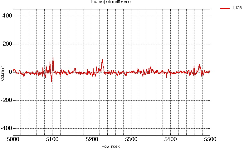
Figure 12. Intra-projection difference corresponding to Fig. 11a.
Figure12b. difference computation principle.
Once these intra-projection differences computed, one can compute inter-projection difference, based on the same idea.
And finally, an entropy based coding technique could be applied on each projection (such as LZW, huffman...)
| Original Image : (256x256x8bpp) | 524 288 bits | ||
| Entropy computation
: intra-projection difference : Difference 128-129 : Difference 129-130 : |
33406 bins 33406 bins 33406 bins |
5,7 bpb 3,86 bpb 3,63 bpb |
190 414 bits 128 947 bits 121 263 bits |
| Total (3 projections):
Compression rate: |
440 624 bits 84 % |
||
| Total (2 projections):
Compression rate: |
311 677 bits 59 % |
Applying a segmentation algorithm on the projections could significantly improve the intra-projection coding.
This would allow to separate the different series (as shown in fig. 11).
2.2. Haar Mojette transform
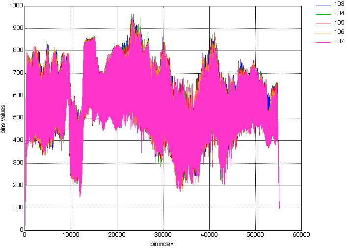 Figure 12a. Full Dirac Mojette |
|
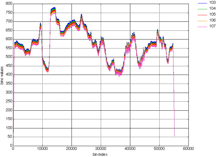 Figure 12b. Full Haar Mojette |
|
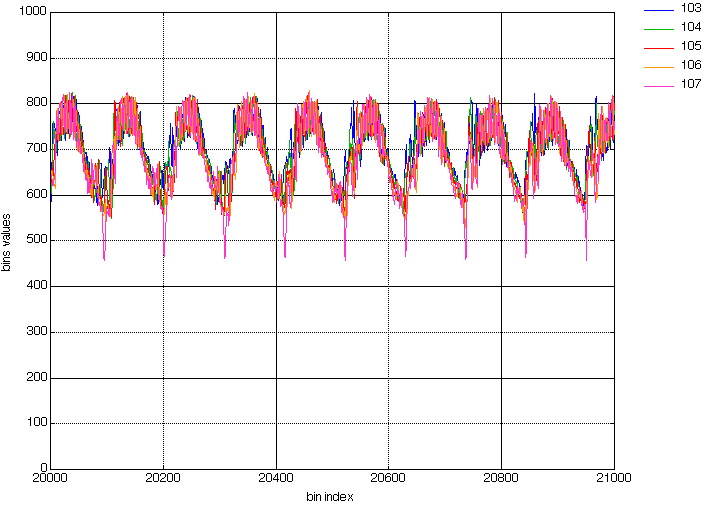 Figure 12c. First zoom on the dirac projections (20000 to 21000). |
|
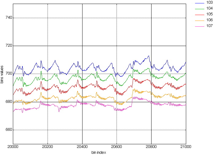 Figure 12d. First zoom on the Haar projections (20000 to 21000). |
|
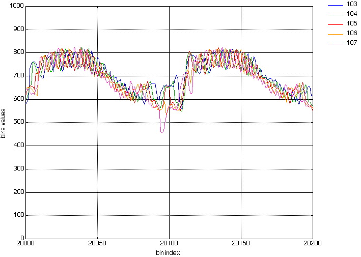 Figure 12e. Second zoom on the dirac projections (20000 to 20200). |
|
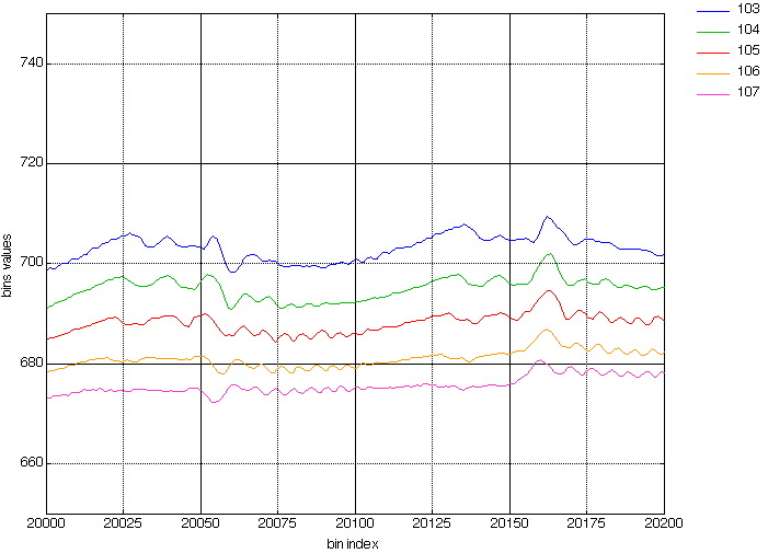 Figure 12f. Second zoom on the Haar projections (20000 to 20200). |
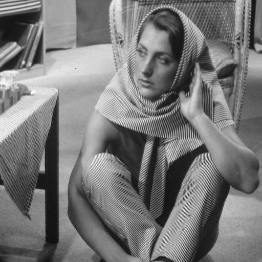
Figure 12 shows the projections for image "barbara" (512x512), and for angles (1,103) (1,104) (1,105) (1,106) (1,107).
The left columns shows the Dirac Mojette transform projections, while the right columns stands for the Haar Mojette projections.
See here for the first results on color images.
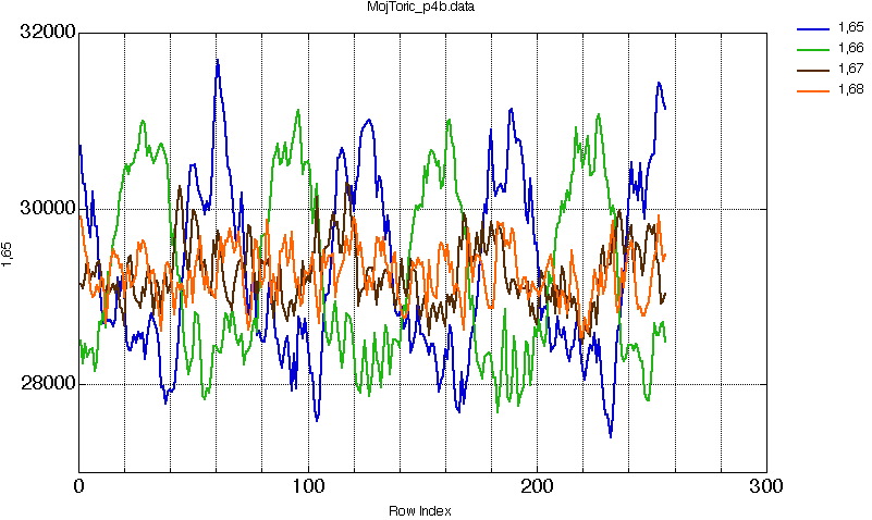
2.3. Finite Radon Transform
The similarities between toric Radon transform projections is not so obvious...
4. References
[1] N. Normand, JP. Guédon, " La transformée Mojette : une représentation redondante pour l'image". Comptes rendus de l'accadémie des Sciences de Paris, Informatique théorique, pp. 123-126, Jan 1998.
[2] I. D. Svalbe, Sampling properties of the discrete radon transform. Discrete Applied Mathematics 139(1-3): 265-281 (2004)
[3] P. Verbert, V. Ricordel, JP. Guédon, Analysis of Mojette transform projections for an efficient coding, 5th International Workshop on Image Analysis
for Multimedia Interactive Services, WIAMIS 2004.
[4] F. Autrusseau, JP. Guédon, Y. Bizais, "Watermarking and cryptographic schemes for medical imaging", SPIE Medical Imaging, Image processing, vol. 5032-105, (8 pages), San Diego California, USA, 15-20 February 2003.
[5] Florent Autrusseau, Benoit Parrein, Myriam Servieres, "Lossless Compression Based on a Discrete and Exact Radon Transform: A Preliminary Study", accepted for publication in the IEEE International Conference on Acoustics, Speech and Signal Processing, ICASSP'06, Toulouse, France 2006.